In the previous post, Introduction to batch processing – MapReduce, I introduced the MapReduce framework and gave a high-level rundown of its execution flow. Today, I will focus on the details of the execution flow, like the infamous shuffle. My goal for this post is to cover what a shuffle is, and how it can impact the performance of data pipelines.
The Cost of Moving Data
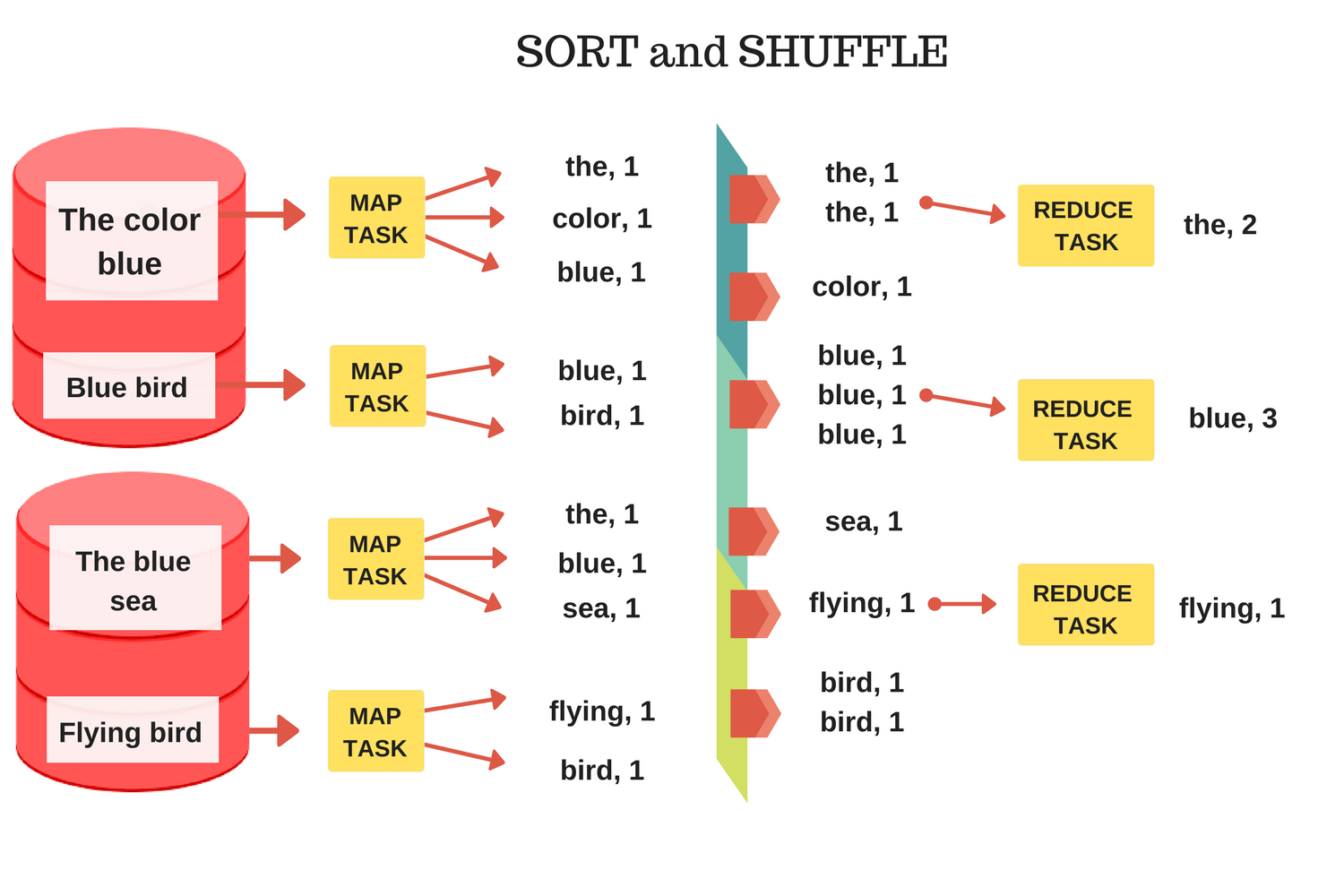
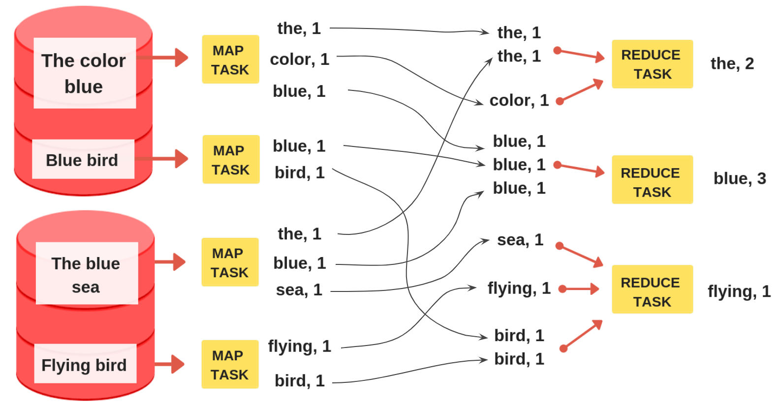
The figure below contains an example of how the counting words problem works in a MapReduce framework. We saw, in the previous post, that the number of mappers is fixed – it is equal to the number of partitions we have for our input data. The number of reducers, on the other hand, is defined by us, the programmer. Each reducer can get data from any of the mappers. In a distributed system, this moving of data between nodes results in network, memory and disk costs which slow down the computation. To understand this cost and how to use it to improve our computation time, we need to understand what exactly happens during the data movement phase (the sort and shuffle phase).
Shuffle
We know that the reducers get the data from any number of mappers, which means that some reducers might not get any data, while others might get data from all the mappers. This spaghetti pattern (illustrated below) between mappers and reducers is called a shuffle – the process of
This is an expensive operation that moves the data over the network and is bound by network IO. If you remember from the Introduction to batch processing – MapReduce post, we learned that the whole point of MapReduce is to minimize data movement by sending our code (map and reduce functions) to the nodes containing data. This naturally leads to the conclusion that shuffles could be a serious bottleneck for MapReduce-based data pipelines. This shows the importance of properly partitioning the data, defining the number of reducers and even sometimes repartitioning the input data to speed up computation. Unfortunately, data transfer is not the only cost of a shuffle. During the shuffle phase, data is sorted and also sometimes written to disk.
Disk
Classical MapReduce frameworks like, the one found in Hadoop, would use disk storage to write out their output results and temporary buffers. This would make it easy to chain multiple MapReduce jobs to create complex pipelines. However, this design means that a large and complex MapReduce data pipeline would also acquire huge disk IO cost, making it even slower. This has inspired other distributed computation frameworks that prefer to keep data in-memory like Spark.
Sorting
Each paragraph so far explained a resource cost in a MapReduce-based data pipeline, as well as why it is there in the first place. What about sorting?
The reduce phase consists of reducers applying a function to reduce incoming data. This function is applied to a chunk of input data with the same key. One easy way to implement this is, well… just sort the input data by keys. This way, the reducer can easily iterate over the sorted data and apply its function. Because the reducer can get data from multiple mappers, each mapper sorts its outputs locally and sends the sorted chunks to the reducers. Reducers then just merge the sorted chunks. This is called Merge sort and it is one of the most famous sorting algorithms in big data and distributed systems. It falls into a class of external sorting algorithms which can easily handle massive amounts of data (just like our MapReduce-based data pipeline).
Conclusion
MapReduce is a convenient abstraction and a robust model to process large amounts of data in a distributed setting. It uses the disk to store outputs, and while it is slower than its in-memory competitors, it allows the data pipeline to process huge amounts of data. Processing hundreds of terabytes in a system like this, isn’t a problem. It will do the job, albeit slow, even with a small number of nodes. Processing the same data in a system like Spark might result in faster processing time, but also most likely require a significant increase in either node count or cost per node giving the increase in RAM memory.